“The Elements of Statistical Learning” 교재 2장의 figure들을 python을 이용하여 작성해보았다.
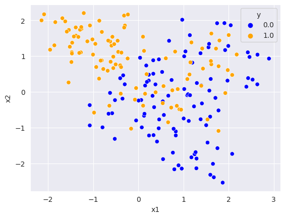
Sample Distribution (Scenario2)
이진 분류 데이터셋으로 각 클래스에 속할 확률은 50%이다. 각 클래스마다 0.1의 확률로 $\mu_k$를 뽑아 $\mathcal{N}(\mu_k, I/5)$로부터 샘플링을 한다. 클래스마다 $\mu_k$의 분포는 다음과 같다.
$ \mu_1^{(blue)}, …, \mu_{10}^{(blue)} \sim \mathcal{N}([1,0]^T, I), \ \mu_1^{(orange)}, …, \mu_{10}^{(orange)} \sim \mathcal{N}([0,1]^T, I) $
(실습 코드)
blue_classes_mean = np.array([1,0])
orange_classes_mean = np.array([0,1])

mu_blue = stats.multivariate_normal.rvs(mean=blue_classes_mean, cov=1,size=10)
mu_orange = stats.multivariate_normal.rvs(mean=orange_classes_mean, cov=1,size=10)


mu_0 = mu_blue[np.random.choice(10,1),:].reshape(2,)
X = stats.multivariate_normal.rvs(mean=mu_0, cov=np.eye(2)/5,size=10)

for i in range(9):
    idx = np.random.choice(10,1)
    mu_i = mu_blue[idx,:].reshape(2,)
    tmp = stats.multivariate_normal.rvs(mean=mu_i, cov=np.eye(2)/5,size=10)
    X = np.concatenate([X,tmp], axis=0)

for i in range(10):
    idx = np.random.choice(10,1)
    mu_i = mu_orange[idx,:].reshape(2,)
    tmp = stats.multivariate_normal.rvs(mean=mu_i, cov=np.eye(2)/5,size=10)
    X = np.concatenate([X,tmp], axis=0)

y = np.zeros((200,1)).reshape(-1,1)
y[100:] = 1
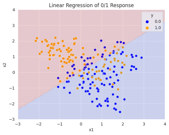
OLS
선형 모델 $Y=X^T \beta$를 가정하여 L2 loss function을 사용한다면, $ \beta^* = [\mathbb{E}(XX^T)]^{-1}\mathbb{E}(XY) $가 최적의 파라미터이다. 대수의 법칙을 통해 $\mathbb{E}(XX^T)$를 $\frac{1}{N} \mathbf{X}^T\mathbf{X}$, $\mathbb{E}(XY)$를 $\frac{1}{N} \mathbf{X}^T \mathbf{Y}$로부터 근사가 가능하다.
따라서 Least Square Estimator인 $\hat{\beta} = (\mathbf{X}^T \mathbf{X})^{-1}\mathbf{X}^T\mathbf{Y}$로 최적의 파라미터를 근사한다. 분류 문제이므로 예측값이 0.5이상이면 1, 미만이면 0을 결정경계로 삼는다.
(실습 코드)
x0, x1 = np.meshgrid(
        np.linspace(-3, 4, 100).reshape(-1, 1),
        np.linspace(-3, 4, 100).reshape(-1, 1),
    )
X_new = np.c_[x0.ravel(), x1.ravel()]

desinged_X = np.c_[np.ones(len(y)),X]
beta_hat = np.linalg.inv(desinged_X.T @ desinged_X) @ desinged_X.T @ y

X_new_with_bias = np.c_[np.ones([len(X_new), 1]), X_new]
y_pred = X_new_with_bias @ beta_hat
y_pred[y_pred <= 0.5] = 0
y_pred[y_pred > 0.5] = 1

sns.scatterplot(x='x1', y='x2', hue='y', palette=palette, data=df)
plt.contourf(x0, x1, y_pred.reshape(x0.shape), alpha=0.2,cmap='coolwarm')
plt.title("Linear Regression of 0/1 Response")
plt.show()
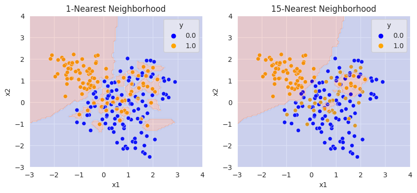
KNN
knn에서 테스트 포인트 $x$에 대해 예측값은 $\hat{f}(x) = \frac{1}{k}\sum_{x_i \in N_k(x)}^N y_i$ ($N_k(x)$는 훈련 데이터셋에서 $x$와 가장 가까운 k개의 데이터 포인트)이다.
마찬가지로 L2 loss를 사용한다면, $N$과$k$가 충분히 크고 $k/N$이 0으로 수렴한다면, 대수의 법칙을 이용하여 $\hat{f}(x)$는 조건부 기댓값으로 수렴함을 보일 수 있다.
(실습코드)
class KNearestNeighbor(object):
    def __init__(self):
        pass

    def train(self, X, y):
        self.X_train = X
        self.y_train = y

    def predict(self, X, k=1):

        num_test = X.shape[0]
        num_train = self.X_train.shape[0]
        dists = np.zeros((num_test, num_train))
        dists = np.sqrt(np.sum(self.X_train**2, axis=1) + np.sum(X**2, axis=1).reshape(num_test,1) - 2*X.dot(self.X_train.T))

        return self.predict_labels(dists, k=k)

    def predict_labels(self, dists, k=1):
        num_test = dists.shape[0]
        y_pred = np.zeros(num_test)
        for i in range(num_test):
            closest_y = []
            closest_y = self.y_train[np.argsort(dists[i,:])[:k]]
            val, cnt = np.unique(closest_y, return_counts=True)
            y_pred[i] = val[np.argmax(cnt)] # majority vote in the neighborhood
        return y_pred
classifier = KNearestNeighbor()
classifier.train(X, y)
y_pred = classifier.predict(X_new, k=1)
y_pred_15 = classifier.predict(X_new, k=15)

plt.figure(figsize=(10, 4))
plt.subplot(121)
sns.scatterplot(x='x1', y='x2', hue='y', palette=palette, data=df)
plt.contourf(x0, x1, y_pred.reshape(x0.shape), alpha=0.2,cmap='coolwarm')
plt.title("1-Nearest Neighborhood")

plt.subplot(122)
sns.scatterplot(x='x1', y='x2', hue='y', palette=palette, data=df)
plt.contourf(x0, x1, y_pred_15.reshape(x0.shape), alpha=0.2,cmap='coolwarm')
plt.title("15-Nearest Neighborhood")

plt.show()
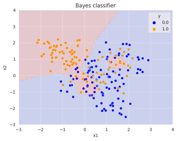
Bayes classifier
0-1 loss를 사용할 때의 최적의 파라미터이다. 모든 $g \in \mathcal{G}$에 대해 $ Pr(g |X=x) $가 최대인 $g$를 구하면 된다. 각 클래스에 속할 확률이 같으므로, 베이즈 정리를 이용하여 $Pr(X=x | g)$가 최대가 되는 $g$를 찾으면 된다.
(실습 코드)
def bayes_classifer(X_new):
    p_blue, p_orange = np.zeros(X_new.shape[0]), np.zeros(X_new.shape[0])
    for i in range(len(mu_orange)):
        p_blue += stats.multivariate_normal(mean=mu_blue[i], cov=np.eye(2)/5).pdf(X_new)
        p_orange += stats.multivariate_normal(mean=mu_orange[i], cov=np.eye(2)/5).pdf(X_new)

    bayes_pred = (p_blue < p_orange)
    bayes_pred = bayes_pred.astype(int)
    return bayes_pred

bayes_pred = bayes_classifer(X_new=X_new)
sns.scatterplot(x='x1', y='x2', hue='y', palette=palette, data=df)
plt.contourf(x0, x1, bayes_pred.reshape(x0.shape), alpha=0.2,cmap='coolwarm')
plt.title("Bayes classifier")
plt.show()
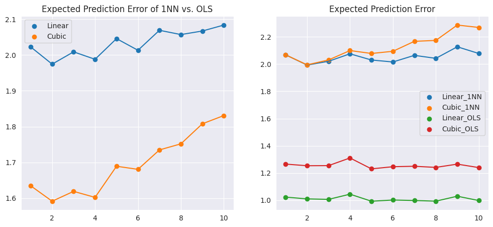
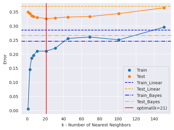
Train/Test Error
200개의 데이터셋으로 훈련을 진행한 후, 새로 10000개의 데이터를 생성하여 테스트 데이터로 사용해 에러를 구하면 다음과 같다.
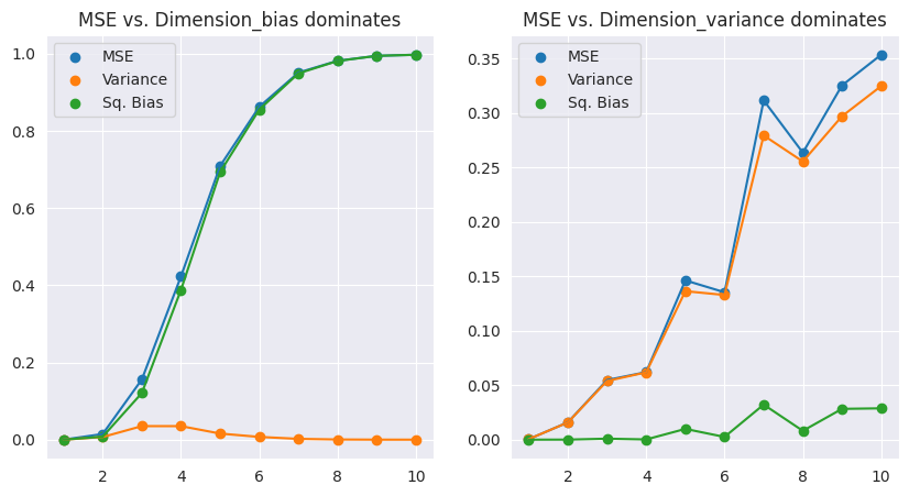
Bias-Variance Decomposition
임의의 데이터 포인트 $x_0$에 대해 $MSE$는 분산과 편향의 제곱으로 분해가 가능하다.
\(\begin{align*} MSE(x_0) &= \mathbb{E}_{\mathcal{T}}(f(x_0) - \hat{y}_0)^2 \\ &= \mathbb{E}_{\mathcal{T}}[f(x_0) - \mathbb{E}_{\mathcal{T}}(\hat{y}_0) +\mathbb{E}_{\mathcal{T}}(\hat{y}_0) - \hat{y}_0)^2 \\ &= Var_{\mathcal{T}}(\hat{y}_0) + bias^2(\hat{y}_0) \end{align*}\)
편향이 MSE를 지배하는 경우의 예시: \(Y = f(X) = \exp(-8||X||^2)\)
분산이 MSE를 지배하는 경우의 예시: \(Y=f(X) = \frac{1}{2}(x_1+1)^3\)